Provisional Version


Profitability of the Universal Postal Service Provider

in a Free Market with Economies of Scale in Collect and Delivery


Prof. Dr. Gonzales d’Alcantara, University of Antwerp and Economic Expert

and Bernard Amerlynck, Freelance Postal Expert


We propose a model for a liberalized competitive postal market with a Universal Service Obligation Provider, the Incumbent, and one Entrant. In this model we take into account the existence of economies of scale in their collect and delivery activities. The study is intended to lead to conclusions about the impact of economies of scale on the postal market in various countries, as measured by the numbers of postal items delivered per person and per year, and by the size of the population. We consider delivery technologies of operators on markets of different sizes, measured both by these two criterions. Variable and fixed costs in the collect and delivery activities are determined by a structural cost model, which has the same form for the Incumbent and for the Entrant. In this latter model we will also pay attention to delivery technologies parameters which differ from country to country, such as the number of delivery points per route stop. Given a definition of the USO, assumptions about demand behaviour and the opening of the market to the Entrant, the calibrated model will compute the impact of the cream skimming mechanism and the graveyard spiral on volume, tariffs, market shares and the cumulative balance of the Entrant needed to finance his delivery network. In a second step, the model will also measure the effects of economies of scale on the financial requirement of the Incumbent in charge of the USO, in case she keeps her tariffs at a constant pre-competition level.


The existence of economies of scale has been recognized in the literature… Key references are K. Jasinski and E. Steggles, (1977), “Modelling letter delivery in town areas”, and, in various Michael A. Crew and Paul R. Kleindorfer edited volumes, John Panzar (1991), “Is Postal service a natural monopoly?”, Cathy Rogerson and William Takis (1993), “Economies of scale and scope and competition in the Postal services”, Michael Bradley and Jeff Colvin (1995), “An econometric model of postal delivery”, Catherine Cazals, M. de Rycke, Jean-Pierre Florens, and S. Rouzaud (1997), “Scale economies and natural monopoly in the postal delivery: comparison between parametric and non parametric specifications”, Robert H. Cohen, and Edward H. Chu (1997), “A measure of scale economies for postal systems”, Bernard Roy (1999), “Technico-economic analysis of the costs outside work in postal delivery”.  All these references show the existence and importance of economies of scale, which clearly exist in the delivery function and to a lesser extent in other activities in the postal value chain. Our purpose is to examine the impact of these economies of scale on the postal market in various countries.  When the market opens and there are economies of scale which differ country by country, what are the long term impacts of a well defined regulatory set-up on tariffs, volumes and market shares in each case? How do economies of scale affect the levels of the tariff differentials between both operators? What is the end-result in each country when scale obviously decreases for the Incumbent with the entry of the competitor, who benefits both from increasing scale and from relatively denser delivery zones, lost by the Incumbent? Which parameters are crucial for the financial requirements of the Entrant, who wants to invest in a delivery network, and for the Incumbent in charge of the USO, when she keeps her tariffs at unchanged – affordable – levels?


The paper will treat two types of model solutions:


a) The regulatory authorities want to achieve a liberalized postal market without giving any subsidies to finance the Universal Service Obligation of the Incumbent. The Incumbent and the Entrant should behave as they would in a situation of competition: both operators determine their tariffs according to their unit costs including the margins to cover their fixed costs. The Incumbent therefore modifies her tariffs so as to keep balanced or break-even accounts.


b) If the Incumbent’s tariffs are required to remain equal to the costs per unit in the base period before the market is opened, the starting situation under monopoly, how large is then the financial loss of the Incumbent, provider of the Universal Postal Service Obligation?


In this contribution we will not take into account the possible inefficiencies of the Incumbent, the obstacles to the access to the market by the Entrant or the transition problems to go from an inefficient and monopolistic to a more competitive market situation.


1.                 The model


The postal market is modelled with two types of customers (j), retail customers and business customers.  The retail customers are afforded special attention by the regulator because they have a high weight in social welfare. They are also characterized by more loyalty to the Incumbent and a less elastic demand than the business customers, who are more cost conscious.  Both customers are assumed to consume one single product, for simplicity the same mix of first and second-class mail services.


There is an Incumbent operator (I) providing services for upstream and downstream. This operator has a Universal Service Obligation. This obligation includes delivering the whole population of the area to be serviced at least one time each day of the week (6 days). The tariff should be an affordable price; therefore tariff will be cost-based. No price-cap has been set-up. The tariff should be the same for all zones of delivery (tariff uniformity). The base period corresponds to a period with a reserved activity for the total volume.


In the first period, when the market is opened, there is an alternative operator - the Entrant (E) - providing competitive services for upstream activity and also able to provide downstream activities. The downstream activity used to be the Incumbent’s reserved activity in the base period, but it is opened to competition in the current period. In other words, in the current period bypass is both technologically and economically feasible for the Entrant.


Total market demand is related to broad substitution possibilities for the customer among different forms of communication. Since in the base period the Entrant is already providing upstream services, new opportunities to create additional mail volume when the conditions and regulations of the downstream activity are changed are not likely. In the model, what is usually called the displacement ratio, s, will be assumed to be equal to 1; i.e. for a given total market demand, an increase of demand of one unit of the Entrant’s service necessarily leads to a decrease of one unit in the demand for the Incumbent’s service. To summarize, within a segment there is perfect substitution between the Incumbent and Entrant’s services. No empirical evidence was found in the literature showing that the displacement ratio for the mail considered is significantly different from 1.


Each country is divided in two delivery zones, the dense or urban delivery zone (U) and the non-dense or rural delivery zone (R).  It is assumed indeed that dense zones are situated in urban areas and non-dense zones in rural areas. Each of these delivery areas is characterized by a grouping index representing the number of delivery points per route stop, in other words the average number of apartments in a building within the urban zone for example. It is assumed that every delivery point (apartment) is occupied by exactly one household, counting 2.6 people in the USA. For the international comparison urban and rural zones are defined following United Nations 2003, Department of Economic and Social Affairs, Population Division, “Percentage population in urban area”. In the USA a proportion of 20.9% of the people live in rural areas, corresponding to non-dense zones: 20.9% of the postal volume is delivered following a lower grouping index and therefore a higher delivery cost. This is true for the Incumbent and for the Entrant, since it depends on the urban and rural organization of the country.


Combining these elements, there are four different segments served by postal service providers: following the customers, where the market shares depend on customers behaviour, and following the density of delivery, where the market shares depend on unit cost differences. 


a)      Demand model


Exactly as d’Alcantara and Amerlynck (2004), there are two steps in the demand model: the first is related to possible substitutions and complementarities of Mail with respect to other communication media on the broad market. The second is related to the Mail customer’s behaviour, given the total mail volume he has determined as his demand. The first is a constant elasticity demand model for total mail demand of a customer in a zone, the second a market share model for each customer, determining the substitution between postal service providers within customers’ market demand, assumes two coefficients: a loyalty coefficient and elasticity.  One defines a customer loyalty percentage as the percentage of the Incumbent’s tariff that a given customer will accept to be higher than the Entrant’s tariff without any decrease in his demand addressed to the Incumbent.   Given the loyalty percentage of a customer and given total market demand of this customer, the elasticity is the percentage change of Incumbent’s volume demanded by this customer and strictly replaced by the Entrant’s product, as a consequence of his percentage discount. Note that there is one elasticity for each customer type, retail and business, and for each destination, urban and rural. The demand model consists of two sets of equations to be solved simultaneously: a total market demand equation for each customer type and the market share equations of the two service providers for their services provided to the two types of customers in the two zones. The structure of these equations is given in the Appendix.


The total market price elasticity of demand for postal services has been assumed to be -.3. The value cannot be rejected in various econometric studies of time series estimation surveyed by Catherine Cazals and Jean-Pierre Florens (2002). At the stage of competing for the market shares, price sensitivity of retail customers is relatively lower then that of business customers. Retail customers are relatively more loyal to the Incumbent’s postal service. The customer loyalty parameters  are considered to be 20% for the Retail Customer and -10% for the Business Customer. The market share elasticity is lower for retail customers (-.75) than for business customers (-1.25). The values of such elasticities are smaller in the case there is a positive loyalty coefficient, which represents a lower tariff sensitivity, and larger in the case there is a negative loyalty coefficient, which represents a higher tariff sensitivity. We have taken the elasticity with zero loyalty / disloyalty to be minus one. Such order of magnitude of the elasticities for all mail categories should not be rejected, when looking at  the values found for first and second class mail separately in various microeconometric demand studies, including their own, surveyed by the same Catherine Cazals and Jean-Pierre Florens (2002).


Figure 1 : Customer behaviour (market share model) : the Switching Function

b) Cost Model


The detailed cost model is presented in the appendix. It is an activity based bottom up cost model. Scale is defined as the number of mail items per person and per year. Population size is explicit in the model but was seen from model solutions not to be significant as an additional size factor. The model is mainly making the quantitative assessment of what is variable and what is fixed cost, such as the park and loop delivery round. The fixed costs related to the USO are central to assess the impact of postal market opening.


Services offered require an upstream activity, including collecting, sorting and transporting, and a downstream activity comprising delivering. Our downstream model is taking over the structure defined by Robert H. Cohen, and Edward H. Chu (1997) for the USA and includes street model complements from K. Jasinski and E. Steggles (1977), further applied by Bernard Roy (1999). The postal activity model is divided in the collection, the sorting of the mail, the in-office delivery, representing the sequencing of the mail into delivery routes, transportation and the street delivery. The street delivery decomposes itself into route travel, delivery access time and load time. The route travel represents the walking or driving along the route without stopping to delivery points. Route travel has 4 modes: Foot Delivery (the cost of foot delivery depends only of the number of hour worked by the carrier), Bicycle Delivery (the cost of bicycle delivery depends of the hours worked by the carrier and of the maintenance of the bicycle), Park & Loop Delivery (the cost of the Park & Loop delivery method depends of the hours worked by the carrier and of the maintenance of the car) and Car Delivery (the cost of car delivery depends of the hours worked by the carrier and of the maintenance of the car). The delivery access time represents the time to deviate from the route to access the delivery points. The load time represents the time to place the mail in the mail receptacle of the delivery points.


The fact that each delivery area is characterized by different grouping indices representing the number of delivery points per route stop has a considerable impact on the unit costs of delivery. The cost ratio between rural and urban zone delivery precisely depends on this grouping index. This 
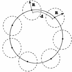
cost differential is the driving element in the cream skimming mechanism. One assumes the average value of this parameter in the rural zone to be equal to 1, as a standard. This is interpreted that in the rural zone one stop corresponds to a one family house. The average value of this parameter in the urban zone of the USA was estimated to 2.12 in 1993 (see appendix). As a standard the value will be fixed at 2.


The United States of America is the largest scale country and will be considered as standard for the calibration of the cost model. The costs of a number of other countries are derived from a set of country related variables. These data have still to be completed, especially for specific postal data. The variables used are the following: Total population (United Nations 2003 -Department of Economic and Social Affairs - Population Division), Percentage population in urban area (United Nations, idem), Employed Labour Cost Nace I (Eurostat, Labour cost survey 2000), Mail items delivered per person and per year, used for scale (UPU 2000), share of Retail customer’s mail in the market (Postal, assumed to be 50%), delivery frequency (UPU 2000), average household size, % foot, bicycle, Park&Loop and car delivery modes (postal), exchange rate in purchasing power parity (1993 PPP compared to USD; for USA PPP in 2003 data compared to euro zone), Consumers price index (Eurostat), Self-employed cost ratio (assumed to be 50%). Medium scale countries can be compared to countries such as Norway and France. Italy and Greece are examples of small scale countries.


When introducing a country, we started with the USA; we need population size and the number of mail items per person and per year. The statistical data about USPS are taken from Cohen and Chu (1997). The values for the parameters are the following:

Delivery network: Delivery points per route: URBAN 488, RURAL 469. Grouping index: RURAL 1 delivery points/stop. Delivery speed: foot  4 km/hour; bicycle 15 km/hour; park&loop car 35 km/hour. In between stop distance: foot 20 m; bicycle 100 m;  park&loop car 300 m.

Vehicle cost ratio 0,02. Entrant delivery frequency 3 delivery/week.

Entrant starting geographic coverage: URBAN 10,0% RURAL 0,0%


c)      The USO, Entrant’s behavior and the dynamic tariff modeling


The Universal Service Obligation is one of the major exogenous factors of the model we have constructed. We have defined the following USO to be imposed by the Regulator on the Incumbent. This allows answering the major question considered in this study, namely the impact of economies of scale on the postal market in different countries. The USO is as follows:


i.             Daily distribution frequency (6 times)

ii.             Constant Quality (J + 1, J + n arrival percentage, which is related to frequency)

iii.             Distribution to all customers (retail and business, urban and rural zones)

iv.             Cost based tariff uniformity for end-to-end  and for access

v.             Affordable tariffs (interpreted as keeping its present value for the Retail customers)

vi.             Availability (interpreted to  be existence)


The Entrant is given the objective to become the first market player and therefore to deliver as much mail as possible without endangering his competitiveness. Therefore the Entrant will invest in a delivery network, as long as his cost to deliver mail is lower than the access tariff of the Incumbent. Between two periods, the Entrant has the ability to decide to extend its delivery network or not. The new geographic coverage of the Entrant delivery network will be equal to the collected market share of the previous period. This justifies the financial losses made by the Entrant during the first periods of entry. This amount tends to zero when investment tends to zero and the cumulated amount to be financed corresponds to the value of the capital needed to establish his business. Note that once the network has been extended, it is not possible to reduce it afterwards. The Entrant does not have any Universal Service Obligation.


Entrant’s behaviour is determined in the following way, all of the parameters being parameters and can be changed in the calibration:


i.         Distribution 3 times per week (different in quality level then Incumbent)

ii.       Same cost structure and parameters as the Incumbent

iii.      Uses self-employed at 50% of national hourly wage cost

iv.     Different full cost tariffs for dense and non-dense zones

v.       A starting investment in a delivery network in view of distributing in the urban (dense) zones a share of 10% of the corresponding total volume of the urban zone

vi.     Access to the Incumbent’s delivery network for the residual volume, namely the volume

      above his bypass potential

vii.    Invest in own delivery network, according to yearly decision made in advance, an amount

capable to deliver the amount collected in excess above his existing bypass capacity of the    precedent period, only if his delivery cost is lower than  the access tariff of the Incumbent.


Access pricing of the Incumbent is set at an access cost level, the average variable delivery cost including fixed costs plus a standard overheadIt would be possible to make a sensitivity analysis of the model results using a  wider range of well-known access pricing methods, including those of the form that Michael Crew and Paul Kleindorfer and the Toulouse School have indicated as more efficient (of the DAP form).


The demand model is solved using iterative method. The model iterates until finding the market equilibrium. The competitive process starts with the entry of the competing operator and the dynamic tariff determination works as follows: The tariffs are set and fixed prior to the iterations. The demand of the previous period is the starting point. All tariffs are cost based. The Incumbent takes the total cost incurred in the previous period without the eventual cost of Entrant re-injection and considering the total mail volume collected in the previous period. The unit cost obtained is set as the Incumbent tariff of the current period. Like its end-to-end tariff, the Incumbent’s access tariff equals its unitary distribution cost, including the fixed costs and a general expense margin. The Incumbent satisfies tariff uniformity, both for end-to-end and for access. As the mail volume re-injected by the Entrant is not predictable by the Incumbent, it has been chosen to compute her end-to-end tariffs only taking into account her end-to-end volume. The unit cost of the Entrant is computed likewise but including the cost of re-injecting his mail in the Incumbent’s network and considering all his mail volume collected.


i.          The starting point is the monopoly situation: volumes per customer and per zone

ii.         Cost based tariffs are fixed by Incumbent, according USO and following equations defined in Appendix

iii.         The Entrant determines his volume objective, unitary cost following the cost model (see Appendix), tariffs per zone, volume delivery objective and corresponding investment in his network

iv.        Cream skimming competition is simulated by the demand model. Equation (1) of  the Appendix gives a new market average tariff. The global mail demand is updated by the equation (2). Then total mail volume is computed. Then, a new value is obtained for  from the equation (3). The value  is the complementary of the present demand

v.         When the market equilibrium is reached, the mechanism yields end of year volumes and market shares

vi.        On the basis of the volume and market share results, the Entrant decides his distribution network for next period. He wants to distribute what he was not able to distribute and had to re-inject through access of the Incumbent’s network a higher access tariff

vii.        New cost based tariffs are set

viii.              Go to point iv, if % variation of one tariff or demand is higher then convergence criterion e, this means as long as market equilibrium is not reached  .


The calculation is stopped after 10 periods (i.e. 10 years), since it marginal tariff changes become smaller then a small convergence criterion after 5 or 6 periods.


Clearly the model describes the Entrant taking away mail through bypass: this erodes Incumbent’s economies of scale in those zones in which bypass occurs.  Such erosion changes the volumes delivered by each operator in each zone and this determines average costs of both operators, according to the zones in which bypass occurs.  The zone-specific impact of the Entrant is eroding delivered Incumbent mail volumes, first in the dense low-cost zones, and therefore diminishes her economies of scale and therefore leads to her tariff’s increase in view of restoring her eroded profitability. In the case of the Entrant, the increase of his volume decreases his unit cost because of increased economies of scale but the increase of his volume in less dense zones increases his unit costs.


d)      Results


Let’s first summarize the assumptions made to calibrate our model about the standard country, the customers, the competitor and the access regulation. One introduces the number of items delivered per person and per year and the population for the USA, the standard country. Its other parameters are:

Cost elements: Urban area = 80 %. Labour cost per hour = 20,32 €. Retail ratio = 0,5. Delivery frequency Incumbent = 6. Household size = 2,6. Foot delivery = 6%. Bicycle delivery = 0%. Park & Loop delivery = 39%. Car delivery = 55%. Exchange rate € per dollars (2003) = 0,88... CPI (2003) = 1,40... Grouping index rural = 1. Grouping index urban = 2.

Retail and Business Customers: Market elasticity = -0,3. Retail loyalty = 20% Business loyalty = -10%. Retail substitution = -0,75.  Business substitution = -1,25. Sigma = 1.

Competitor: Freelance cost ratio= 0,5. Delivery frequency Entrant = 3. E starting coverage urban = 10%  E starting coverage rural= 0%.

Price regulation: Access pricing = accessed cost. Including other costs = Yes. Tariff uniformity on access = Yes


With these values the process converges. In a second step the values of the Mail delivery Density are introduced corresponding to fixed intervals of 50. In this way one obtains results corresponding to the sizes of most country: in each case the model follows a process where scale obviously decreases for the Incumbent with the entry of the competitor, and when the Incumbent looses dense urban zones because of her high uniform tariffs. The Entrant benefits both from increasing scale and from cream skimming the relatively denser delivery urban zones, lost by the Incumbent. In Table 1. “Model Results per Country Scale” countries are placed in view of the corresponding scales. After 5 or 6 periods the model always converges, but the period reported is period 10. One should not interpret these results as final values for the countries since the calibration of the data used should still be considerably improved. However the large variations obtained in the results are of interests to understand the impact of economies of scale.


1° Solutions with break-even tariffs for the Incumbent


When the market opens and with the definition of the USO, what are, according to economies of scale which differ country by country, the long term impacts on tariffs, volumes and market shares? These   variables of the converged model result are shown following the number of mail items per person and per year.


§       Unit cost variation under monopoly (unit cost = 1 for USA)

The cost curve is non-linear. While the medium size countries Norway and France have a 4% and a 10% handicap, Italy and Greece have a 135% and 276% cost handicap.


gU = 2

USA

Norway

Austria-France

Finland-UK

Belgium

IrelandJapan

Portugal

Spain

Italy

Greece

Scale

1,00

0,85

0,70

0,55

0,45

0,30

0,25

0,20

0,15

0,08

Unit costs

1,00

1,04

1,10

1,19

1,29

1,56

1,71

1,95

2,35

3,76


Graphically presented, one has


Figure 2 : Standardized Unit Cost in function of Scale


§         Incumbent tariff variation after competition (Incumbent tariff after competition convergence divided by Incumbent tariff under monopoly)

The tariff increase to be introduced by the Incumbent as a consequence of the arrival of the Entrant, her loss of size and of less costly urban zones, results to be relatively important, but much more so in small size countries: the USA tariff increases by 53% while the French one increases by 72% and the Italian increases by 126%. This corresponds to the price the retail customer has to pay for the USO after the opening of the market.


§         Entrant Urban and Rural tariffs after competition (Entrant tariff in Urban and Rural areas after competition convergence divided by Incumbent uniform tariff under monopoly)

The discount given by the Entrant is considerably higher in small size countries then in large size countries: extremes vary with 66% against 39% in the Urban zones and with 36% against 29% in the Rural zones; this also reflects a relatively more aggressive behavior of the Entrant in the Urban zones of the small countries. Scale is less significant in Rural zones because higher unit costs prevents the Entrant to capture market share.


§       Total volume variation after competition (volume after competition convergence divided by volume under monopoly). The impact of competition on reduced average tariffs and on general communication market substitution is positive and stronger in small scale countries, the extremes varying from a 10% increase to a 25% increase.


§       Entrant Collect market shares on Retail customers after competition

Retail markets are more difficult to be captured by the Entrant then Business markets because of the loyalty of the customers and their lower tariff sensitivity, but small size again is relatively more dangerous for the Incumbent: in the smallest country the Entrant captures 48% of the Retail market share for a 66% discount in the Urban zones and a  36% discount in the Rural zone against 29% in the USA  for a 39% discount in the Urban zones and a  29% discount in the Rural zone.


§       Entrant Collect market shares on Business customers after competition

Business markets are much easier to be captured by the Entrant then Retail markets, because of the readiness of business clients to switch to the Entrant and their higher tariff sensitivity. In small size countries total 100% market share goes to the Entrant. In the large ones the Incumbent only keeps 14% of the business market. Clearly the business market structure has turned upside down with the assumptions made. It is understandable, because, from a methodological point of view, when in reality a 50% market share is reached, there is a duopoly: it is not possible to keep our same model assumptions about the market structure and parameters. For example, a game theoretic model should be used. The Entrant’s labor cost discount assumed would not be realistic. No further study was done about this.


§       Financial resources needed by Entrant to invest into his own delivery network after competition (Entrant’s cumulative profit or account balance after competition divided by Entrant’s revenue after competition). It is interesting to see the impact of the market opening on the financial resources needed by the Entrant to invest into a delivery network: it is obviously related to the importance of the delivery network he has created to take over a high delivery market share from the Incumbent. In the case of Italy this amount corresponds to 105% of the Entrant’s sales; in France 30%;  in the USA only 18%. These results are acceptable in terms of the financial cost generated.


Tableau 1 : Model Results per Country Scale


USA = 1

Norway

Austria-France

Luxembourg

Finland-UK

Belgium

Ireland-Japan

Portugal

Spain

Italy

Greece


1,00

0,85

0,70

0,65

0,55

0,45

0,30

0,25

0,20

0,15

0,08


Unit cost

1,00

1,04

1,10

1,13

1,19

1,29

1,56

1,71

1,95

2,35

3,76


Volume

110%

111%

113%

114%

116%

117%

119%

120%

121%

122%

125%


Tariff Incumbent

153%

160%

172%

177%

188%

193%

206%

212%

219%

226%

240%

Entrant

Urban Tariff

61%

59%

57%

57%

55%

52%

48%

46%

43%

40%

34%

Entrant

Rural Tariff

71%

71%

70%

70%

70%

69%

68%

67%

66%

65%

64%

Entrant Share Retail Collect

29%

31%

34%

35%

37%

38%

41%

42%

44%

45%

48%

Entrant Share Business Collect

86%

89%

94%

96%

98%

99%

99%

100%

100%

100%

100%

Financial Needs Entrant

18%

23%

30%

33%

40%

49%

68%

78%

90%

108%

146%


Unit cost under monopoly is unit cost = 1 for USA scale

Total volume after competition equals volume after competition convergence divided by volume under monopoly

Incumbent tariff after competition equals tariff Incumbent after competition convergence divided by tariff Incumbent under monopoly

Entrant Urban tariff after competition equals tariff Entrant in Urban area after competition convergence divided by tariff Incumbent uniform under monopoly

Entrant Rural tariff after competition equals tariff Entrant in Rural area after competition convergence divided by tariff Incumbent uniform under monopoly

Collect market shares Entrant on Retail customers after competition

Collect market shares Entrant on Business customers after competition

Financial needs Entrant after competition equals cumulative Entrant loss after competition divided by revenue Entrant after competition


Second we show a number of variables of the converged model result according to two dimensions: not only the scale corresponding to the number of mail items per person and per year, but also the mail delivery density given by the average urban grouping index. The average rural grouping index is assumed to be 1. The urban grouping index, the number of delivery points per route,  typically depends on the urban structure of the country, the number and size of apartment buildings compared to one family houses. It appears to be a crucial factor in the results obtained for unit costs. One finds a cost per item going from the cheapest ( = 1) for the standard country, the USA, to 1.31 in France and to 3.35 in Italy.


For the USA, with an urban grouping index equal to 2, this unit cost in standardized terms goes from 1 to 0,90 where the urban grouping index equals 6. For Italy this standardized unit cost goes from 2.35 with the urban grouping index equal to 2 to 1.69 where the urban grouping index equals  6. These unit cost decreases are most important to understand: they influence the impact of liberalization in the different countries as well as the scale.


One can see the unit cost impacts of scale and density in the Figure 3, obtained from model results.


Figure 3 : Unit costs as a function of scale and urban grouping index


One can see that the higher scale (towards 1 in the graph), represented by the number of items per person and per year, and density (towards 12 in the graph), represented by the urban grouping index, the stronger the position of the Incumbent.


Figure 4 shows the average tariff as a function of scale and density (urban grouping index). This is good news since it opening the market is lowering the average tariff, which is a benefit to the customers. The bad news is that the tariff of the Incumbent, delivering the Universal Service to the retail customer, has increased. The market share of the Entrant is mostly concentrated in the business sector.


Figure 4 : Average tariff as a function of scale and density (urban grouping index)


Figure 5 shows that in the dense or urban zone the Entrant has taken important market shares, the larger when scale and density (urban grouping index) decrease. It is a paradox that the Entrant has a more difficult time to win market shares when density increases. It can be explained because there is uniform tariff constraint on the Incumbent, which implies a relatively lower uniform tariff because delivery costs in the urban zones are lower. This is why the Entrant abandons his rural network almost everywhere, except when the grouping index is small (relatively high delivery costs).

Figure 5 : Coverage of the Rural zone by the Entrant as a function of scale and urban grouping index


Figure 5 : Entrant’s Retail Market Share as a function of scale and urban grouping index


Figure 5 show the market shares obtained by the Entrant in the Retail markets. A higher urban grouping index makes the competitive position of the Entrant more difficult and results in lower market shares: In the USA 29% of the Retail market goes to the Entrant with gU = 2 and 24% with gU = 6. Similarly in the USA 86% of the Business market goes to the Entrant with gU = 2 and 77% with gU = 6.


2° Constants Incumbent tariff solutions

Let us now find another set of model solutions in the case the Tariffs of the Incumbent are not allowed to change compared to their pre-market opening level. The idea is to have an estimation of the financial requirement needed by the Incumbent to deliver the USO, while the Entrant is taking over part of the market share, starting with the dense mail delivery zones. Compared to the first set of model solutions, the Entrant modifies his behavior and decides not to take any market share as soon as his unit costs go beyond the Incumbent’s tariff. The results are given for the urban zone, where the grouping index equals 2. The USA requires a financial compensation of 17% of its revenues while Italy requires 73%. Clearly the result shows scale is a crucial factor.


Figure 6 : Financial need of Incumbent at constant Tariffs in % of own sales


The numerical results are sensitive to many factors which can be modified in the model:


i.         Demand sensitivity: sigma , epsilon, matrix of loyalty parameters X and elasticities

ii.       USO definition: uniform tariffs for retail / business

iii.      Labor factor cost discount of the Entrant (50% used in the calibration)

iv.     Distribution frequency of Entrant

v.       Retail customer ratio

vi.     Access tariff rule: avoided cost / accessed cost, with  / without other cost margin (uniform accessed cost including other cost margin used in the calibration)


CONCLUSIONS


In our previous study about economies of scale and the graveyard spiral in the Postal sector, we showed from a calibration approach that the order of magnitude of the financial losses caused by opening  the postal market are a function of the scale of the Postal Delivery Activity of the Operators. Crucial determinants of these results were the constant tariff of the Incumbent and the assumed annual fixed cost her USO. In the absence of a reserved activity therefore, finances from Government subsidies or a Compensation Fund, necessary to cover the USO, should be a function of the scale of the postal delivery activity of the Company in charge of the USO in each country.


This study calculates economies of scale from a bottom up collect and delivery cost model. There is a complete model wherein a large amount of parameters have to be introduced to fit with the postal situation in each country. This model was used using the data from the USA and USPS: these data correspond to the country with the largest scale postal network observed. The model is standardized according to this reference and allows introducing the observed data for all other geographical units and operators. Sensitivity analysis can also be performed.


The impact of opening the postal market depends from scale for many reasons: not only because of the total market tariff elasticity of the total demand for mail, which will determine the total volume of mail demanded, but also from the market shares of each operator, corresponding to the equilibrium of the competitive market, since these market shares will determine economies of scale and average unit costs for the operator. Also the geographic distribution of mail delivery density, the distribution of Urban and Rural zones, is a crucial factor to know what will be the impact of liberalization in each country. In a nutshell we can say:


         A detailed structural and bottom up model measures the impact on unit costs, tariffs, volumes, market shares and financial balances of opening the postal market, with a USO for the Incumbent of any country, for which the parameters are introduced.


         The unit mail costs, after opening the postal market in a country with a USO for the Incumbent, decrease with scale and with urban mail delivery density.


         Incumbent’s increase in tariff to be decided for break-even is higher in small scale countries: this will provide more opportunity for the Entrant to benefit from a tariff discount. It is also higher in less dense countries.


         The financial loss of the Provider of the Universal Postal Service Obligation, if she is not allowed to increase her tariff, is higher in small scale countries then in large scale ones.


         It is not valid to generalize conclusions about market opening in large scale and less dense countries, such as the USA, for European countries:

-          If a break-even Tariff increase of 53% (Cohen 2004 mentioned up to 78%) could be acceptable for the Postal Rate Commission, increases of more then 100% are difficult to accept for a Regulator in European countries in view of affordability.

-          Alternatively, to finance the cost of the USO for an amount of 17% of sales (USA) is not comparable to orders of magnitude of 40% up to 80% in European countries.


         The market shares of the Entrant become higher in small scale countries and he needs more financial capital to finance the development of his delivery network, in order to bypass the Incumbent’s network in small scale countries.


         In countries with a higher grouping index it is more difficult to compete for the Entrant because there is uniform tariff constraint on the Incumbent, which implies a relatively lower uniform tariff because delivery costs in the urban zones are lower. This is why the Entrant abandons his rural network almost everywhere, except when the grouping index is small (relatively high delivery costs). This is why the Entrant abandons his rural network almost everywhere, except when the urban grouping index is small (relatively high delivery costs).


Technical Appendix

General assumptions


Following the approach of Cohen and Chu (1997), the postal activity will be divided in the mail processing, representing the collection and the sort of the mail, the transportation, the in-office delivery, representing the sequencing of the mail into delivery routes, and the street delivery. The street delivery decomposes itself into route travel, delivery access time and load time. The route travel represents the time it would take to walk or drive the route without stopping to delivery points including the cost of vehicles. The access time represents the time to deviate from the route to access the delivery points. The load time represents the time to place the mail in the mail receptacle of the delivery points.


Each country is divided in two delivery zones, urban (U) and rural (R).  Each of these delivery areas is characterized by a grouping index (gz) representing the number of delivery points per route stop, in other words, within an urban area z, the average number of apartment in a building. It is assumed that every apartment (delivery point) is occupied by exactly one household. The 2003 Urban and rural areas report from the Department of Economic and Social Affairs of the United Nation Organization[1] provides for each country the population living in these two zones, according to the national definition.  The definition of these zones varies from country to country.


Two operators, the Incumbent (I) and the Entrant (E) collect, sort and deliver the mail. The Entrant decides of the geographic coverage (gcEz) of its delivery network in the zone z. The Entrant collect network is proportional to its delivery network. The Entrant has the ability to hire self-employed. These differences will produce substantial savings in the entrant cost structure.


The hourly labor cost for the Incumbent has been taken as the average labor cost of the Transport, storage and communication section (NACE code I, see Paternoster (2002)), . Assuming a self-employed labor cost ratio of 0,5, one have


Demand model


The symbols used for the variables of the model, in the current period and in the previous period (variables with a ^ above the symbol) are the following, given that:


Superscript j{retail, business} represents the two customer segments

Subscript {urban, rural} represents the two destination zones


Quantities:

= customer j’s demand for postal service in zone z from the Incumbent

= customer j’s demand for postal service in zone z from the Entrant

= customer j’s total demand for delivery zone z


The following identities hold:                                                                       


Tariffs:

=   Incumbent's tariff for providing postal service in zone z for customer j

= Entrant's tariff for providing postal service in zone z for customer j

=    Average market price in delivery zone z for customer j

=   Incumbent's average price in delivery zone z

=   Entrant's average price in delivery zone z


The average market prices per zone and per customer  in view of the requirement of non-price discrimination are defined by the following identity:                     (1)

            Exactly as d’Alcantara and Amerlynck (2004), one assumes a constant elasticity demand model for total market demand of a customer in a zone, with the average market price elasticity of total demand for customer j denoted:                                                     (2)

Similarly, the market share model for each customer, determining the substitution between postal service providers within customers’ market demand, assumes two coefficients: a loyalty coefficient and elasticity.  One defines customer loyalty percentage  as the percentage of the Incumbent’s tariff that customer j will accept to be higher than the Entrant’s tariff without any change in his demand addressed to the Incumbent in zone z.  Given the loyalty percentage  and given total market demand of this customer in this zone, the elasticity, denoted, is the percentage change of Incumbent’s volume demanded by customer j in zone z and replaced by the Entrant’s product, as a consequence of his percentage discount. The market share or market entry equations of the Entrant write:

                                                                                        (3)

Note that there is one elasticity for each customer type j{retail, business} and for each destination {urban, rural}. The demand model consists of two sets of equations to be solved simultaneously: a total market demand equation for each customer type and the market share equations of the two service providers for their services provided to the two types of customers in the two zones.

The cost model

As the US postal market is described as the market where the economies of scale are maximal, the United States Postal Service cost data are used as a base case and standard for the cost of the operators of all countries.


1.  Collection (C)


This activity does not depend on the mail volume. One has estimate that 58% of the mail processing cost described in Cohen and Chu (1997) is related to the collection, and is therefore fixed. This cost is adjusted from 1993 USPS similar cost using the total quantity of mail collected under monopoly situation in the measured country.

For the Incumbent,

MPUS(1993) is the actualized 1993 mail processing cost incurred by USPS, and QUS(1993) is the 1993 mail volume of USPS.


From a structural cost model, one deduced that the collection cost is composed of 72% of labor cost. Assuming a self-employed labor cost ratio of 0,5, one has for the Entrant,

where POPz is the population residing in zone z, and POP is the total population.


2. Sorting (S)


This activity is fully variable. If Qo is the volume that the operator o has collected, one has for the Incumbent,

MPUS(1993) is the actualized 1993 mail processing cost incurred by USPS, and QUS(1993) is the 1993 mail volume of USPS.


From a structural cost model, one deduced that the sorting cost is composed of 23% of labor cost. Assuming a self-employed labor cost ratio of 0,5, one has for the Entrant,


3. Transportation (T)


The part of the transportation cost which is not directly related to delivery is variable, while the transportation cost related to the delivery activity is fixed.

One have then to remove from the 1993 USPS transportation cost described in Cohen and Chu (1997) the delivery round transportation costs incurred by USPS at that time (DRTUS(1993)).  If Qo is the volume that the operator o has collected, one has for the Incumbent,

TUS(1993) is the actualized 1993 transportation cost incurred by USPS, and QUS(1993) is the 1993 mail volume of USPS. The estimation of DRTUS(1993) is described below.

From a structural cost model, one deduced that the transportation cost is composed of 39% of labor cost. Assuming a self-employed labor cost ratio of 0,5, one has for the Entrant,


4. In-office delivery (IOD)


The cost of this activity depends of the mail volume each operator actually delivers. One assumes that there is no difference between mail sequencing in urban area or rural area. If  is the volume that the operator o has to deliver in the zone z, one has for the Incumbent,

IODUS(1993) is the actualized 1993 in-office delivery cost incurred by USPS, and QUS(1993) is the 1993 mail volume of USPS. From a structural cost model, one deduced that the in-office delivery cost is composed of 47% of labor cost. Assuming a self-employed labor cost ratio of 0,5, one has for the Entrant,


5. Street delivery: Route travel (RT)


The route travel is a fixed cost depending of the delivery frequency (df), representing the number of delivery per week, and the geographic coverage of the delivery network.


First one estimates the number of routes per delivery zone (rU and rR) using the 1993 USPS data. According to Cohen and Chu (1997), in 1993, there were 164 thousand city delivery routes with 80 millions delivery points and 49 thousand rural routes with 23 millions delivery points.  We obtain then an average of 488 delivery points per urban route (dU), and 469 delivery points per rural route (dR). We take these results as universal.


The geographic coverage of the operator o in the delivery zone z (gcoz) is the percentage of routes actually served by the operator in this zone.

Under the assumption that one delivery point corresponds to one household, and for hs defined as the average number of habitant per household and POPz as the population in the delivery zone z, one has for each delivery zone z:           

Due to the universal service obligation, the incumbent has to serve the entire territory (gcIU + gcIR = 100%). Every route is delivered either by foot, by bicycle, by car or with a park and loop[2] technique. The number of routes served with a specific method in each zone is given using the data available in Bernard, et al. (2002).

Table 2 : Delivery mode by route (in percent of routes)

Delivery method

Route proportion in France

Route proportion in United States

Foot

14%

6%

Bicycle

48%

0%

Park and loop

0%

39%

Car

38%

55%

The car delivery is a typical rural delivery method while the foot delivery is typically urban. The bicycle and park and loop methods are more polyvalent.


We take the same basic data as described in Roy (1999) to model each delivery method cost. A specific model estimating Park & Loop delivery costs will be described below.

Table 3 : Speed of movement and average distance between stops

Delivery method

Distance between stops (ds)

Speed of movement (ms)

Foot

20 m

4 km/h

Bicycle

100 m

15 km/h

Car

300 m

35 km/h


For the vehicle costs per kilometer one assumes the same relative cost estimation as in Roy (1999), namely 50, the ratio between labor cost per hour worked and vehicle costs per kilometer.


Variable gz is called the grouping index in the delivery zone z and represents the number of delivery points per stop, for example a house or an apartment, in zone z, one has the following yearly route time costs for the operator o:


Foot delivery

The cost of foot delivery depends only of the number of hour worked by the carrier.

Bicycle delivery

The cost of bicycle delivery depends of the hours worked by the carrier and of the maintenance of the bicycle. We neglect the last part.

Park & Loop delivery

The cost of the Park & Loop delivery method depends of the hours worked by the carrier and of the maintenance of the car. One assumes that a park & loop delivery round is composed of a single round made by car, and constituted of n parking. Each of this parking is the starting point of a circular delivery round made by foot. Let d be the distance between two parking, this distance is the constant. The total distance traveled by car equals then. Let R be the radius of the pedestrian circular round. The number of possible stops on a pedestrian circular round in zone z is equal to   , where dz represents the average number of delivery points in a pedestrian round in zone z . Making use the basic data described in Roy (1999), the average perimeter of a pedestrian round is equal to   meters. As these delivery rounds are assumed circular, the radius R equals.

This model gives that , one will consider the limit case d = 2R. The average time traveled by foot (movement speed of 4 km per hour) on a park & loop route in zone z equals. While the average time traveled by car (movement speed of 35 km per hour) on a park & loop route in zone z equals. The vehicle cost is computed taking the same relative cost


Figure 7 : Park & Loop delivery round

estimation as in Roy (1999). The yearly cost of a single park & loop delivery route in zone z, including the vehicle cost, is then,


Car delivery

The cost of car delivery depends of the hours worked by the carrier and of the maintenance of the car.


The total route travel cost for the operator o will be


6. Street delivery: delivery Access Time (AT)


The access time is partly fixed and partly variable. As described in Cohen and Chu (1997), this cost depends of the percentage of possible stops that are accessed on a route given by the coverage function (COV). This function is a result of a nonlinear regression model and the coefficient estimated by Cohen and Chu  is used: where b = 0.6587 and PPSoz is the number of pieces per stop in the delivery zone z for the operator o. Variable PPSoz is linked to the volume delivered by the operator o in the zone z () with the following relation,   where PPSz(monopoly) and Qz(monopoly) are respectively the number of pieces per stop and the volume delivered in the zone z in the monopoly situation. In 1993 in the United States, 93% of all possible stops receive mail each delivery day. One uses this data as a reference for the incumbent in a monopoly situation. Therefore,                                    .

The elemental access time cost per stop (at) is derived from the 1993 USPS cost,  where ATUS(1993) is the actualized 1993 access time cost incurred by USPS, #stopUS(1993) is the total number of possible stops on the US delivery network in 1993, and COVUSPS(1993) equals 93%. As in 1993, 80 millions delivery points and 23 millions delivery points are respectively claimed to be served by USPS in urban and rural areas, the number of stops (#stopUS(1993)) is equal to the following .

A short model estimating the grouping indexes in both delivery zones will be described below.

Then one has for the Incumbent,

This activity represents the time of stopping and accessing the delivery point. It is therefore only a labor cost. Assuming a self-employed labor cost ratio of 0,5, one has for the Entrant,


7. Street delivery: Load Time (LT)

The load time cost is fully variable. Then if  is the volume that the operator o has to deliver in the zone z, we have for the incumbent

LTUS(1993) is the actualized 1993 load time cost incurred by USPS, and QUS(1993) is the 1993 mail volume of USPS. This activity represents the time of placing the mail in the receptacle of the delivery points. It is therefore only a labor cost. Assuming a self-employed labor cost ratio of 0,5, one has for the Entrant,


8. Other costs (OTH)


Based on the 1993 USPS data, one has observed that an important share of the total cost is allocated to overheads, namely 24% of the previously described costs. This markup will be added for each operator.

Estimating grouping index

One assumes gUSPSR(1993) equal to 1. In the rural zone one stop corresponds to a one family house. One needs to estimate gUSPSU(1993). In the urban zone one stop averages to a multi family apartment. We derive it from the total USPS route time cost in 1993. From Cohen and Chu (1997) it is deduced that, in 1993, the hourly labor cost for USPS worker was approximately 21,5$. As the delivery frequency obligation in the United States is 6 deliveries per week, one has the following annual route time costs (route time cost is equal to the route travel cost minus the vehicle cost):


The number of delivery routes in 1993 is deduced from the delivery mode repartition described in Bernard, et al. (2002) and from the number of urban and rural delivery routes described in Cohen and Chu (1997).

Table 4 : USPS delivery routes in 1993

Delivery method

Urban zone

Rural zone

Foot

12780

0

Bicycle

0

0

Park & loop

83070

0

Car

68150

49000

Total

164000

49000


The total USPS route time cost in 1993 was 2950 millions $. This will lead to the following identity,

and gUSPSU(1993)=2,12.


Estimation of 1993 USPS delivery rounds transportation costs

One will determine the 1993 USPS cost of transportation directly related to delivery routes. As described above, the yearly cost of transport in delivery routes regarding the delivery mode is the following

From the previous paragraphs, it is known that dU = 488, dR = 469, gUSPSU(1993)=2,12, gUSPSR(1993)=1, dfUSPS(1993) = 6 and LUSPS(1993) = 21,5$.

The number of routes per delivery mode and delivery zones is computed inTable 4.

Actualization of 1993 USPS financial data

The 1993 USPS figures have been converted into euro using purchasing power parity. The actualization was made using national consumer price index evolution. 

References

Bernard, Stephane, Robert Cohen, Matthew Robinson, Bernard Roy, Joëlle Toledano, John Waller and Spyros Xenakis. 2002. In Postal and Delivery Services: Delivering on Competition; edited by M.A. Crew and P.R. Kleindorfer. Boston, MA: Kluwer Academic Publishers.


Bradley, M., and J. Colvin. 1995. “An econometric model of postal delivery”. In Commercialization of postal and delivery services, edited by M.A. Crew and P.R. Kleindorfer. Boston, MA: Kluwer Academic Publishers.


Casals C., M. de Rycke, J.-P. Florens, and S. Rouzaud. (1997). “Scale economies and natural monopoly in the postal delivery : comparison between parametric and non parametric specifications”. In Management change in the postal and delivery industries, edited by M.A. Crew and P.R. Kleindorfer. Boston, MA: Kluwer Academic Publishers


Cazals, Catherine and Jean-Pierre Florens. 2002. “A comparison between cross-section and dynamic data”. In Delivering on Competition, edited by M.A. Crew and P.R. Kleindorfer. Boston, MA: Kluwer Academic Publishers


Cohen, Robert H., and Edward H. Chu. 1997. “A measure of scale economies for postal systems”. In Managing Change in the Postal and Delivery Industries, edited by M.A. Crew and P.R. Kleindorfer. Boston, MA: Kluwer Academic Publishers.


Cohen, R., M. Robinson, G.Scarfiglieri, R. Sheehy, V. Visco Comandini, J. Waller, S. Xenakis. 2004. “The role of scale economies in the cost behaviour of  Posts”,  to be published in the Proceedings of Wissenschaftliches Institut für Kommunikationsdienste GmbH (WIK), 8th Köenigswinter Seminar on Regulating Postal Markets - Harmonised Versus Country Specific Approaches, February 16-18, 2004.


d’Alcantara, Gonzales and Bernard Amerlynck. 2004. “Financial Viability of the Universal Postal Service Provider under Uniform and Cost related Tariffs”. Published in Competitive Transformation of the Postal and Delivery Sector, edited by M.A. Crew and P.R. Kleindorfer. Boston, MA: Kluwer Academic Publishers.


Jasinski, K. and E. Steggles. 1977. “Modelling letter delivery in town areas”. In Computers and operational reseach, Vol 4, pages 287-294. Pergamon Press.


Paternoster, Anne. 2002. Labour Costs Survey 2000: Member States, Statistics in Focus, Population and Social Conditions, Theme 3, 7/2003, Eurostat.


Panzar, John. 1991. “Is Postal service a natural monopoly?” Edited by M.A. Crew and P.R. Kleindorfer. Boston, MA: Kluwer Academic Publishers.


Roy, Bernard. 1999. “Technico-economic analysis of the costs outside work in postal delivery”. In Emerging Competition in Postal and Delivery Services, edited by M.A. Crew and P.R. Kleindorfer. Boston, MA: Kluwer Academic Publishers.


[2] S. Bernard, et al. (2002) : “Park and loop refers to a route where the carrier parks his or her vehicle and serves a group of houses on foot, returns to the vehicle and drives to another location where the process is repeated”